Methods2,101 words, 10 minutes
Bond math from first principles: price, yield, duration, convexity
Price, yield to maturity, Macaulay and modified duration, and convexity derived and coded from scratch, then applied to the Treasury par curve of 2026-09-09.
Every number a bond desk quotes, from a price to a DV01, comes out of one sum: the present value of the cash flows. This article builds that sum in about forty lines of standard-library Python, differentiates it twice, and checks each derivative against a finite difference before trusting it. It then applies the result to a real curve, the eleven Treasury constant-maturity yields the Federal Reserve publishes and FRED redistributes, as they stood on 2026-09-09. The dataset back to 2000 and the script are attached; every figure below is printed by that script, and nothing here is advice about owning any bond.
Where the yields come from, and why they price at par
The H.15 release describes the series precisely: yields on Treasury nominal securities at "constant maturity" are "interpolated by the U.S. Treasury from the daily yield curve for non-inflation-indexed Treasury securities", a curve that "is based on the closing market bid yields on actively traded Treasury securities in the over-the-counter market." The values are "read from the yield curve at fixed maturities, currently 1, 3, and 6 months and 1, 2, 3, 5, 7, 10, 20, and 30 years", which, as the release notes, "provides a yield for a 10-year maturity, for example, even if no outstanding security has exactly 10 years remaining to maturity."
The Treasury's own methodology page adds the property that makes the arithmetic below clean: "The Treasury's official yield curve is a par yield curve derived using a monotone convex method", built from "indicative, bid-side market price quotations (not actual transactions) for the most recently auctioned securities obtained by the Federal Reserve Bank of New York at or near 3:30 PM each trading day." A par yield is the coupon rate at which a bond of that maturity would price at exactly face value. So a hypothetical 10-year bond carrying a 4.83 percent coupon, the DGS10 print for 2026-09-09, prices at 100.0000 when discounted at 4.83 percent. That is not a coincidence the script discovers; it is what the series means, and the script asserts it as a self-check.
Two conventions follow from how Treasuries pay. TreasuryDirect states that "Notes pay a fixed rate of interest every six months until they mature", so the coupon frequency is two and yields compound semiannually. The three bill maturities carry no coupon, so we treat them as single payments discounted at the quoted investment-basis yield with the same compounding; the price of a six-month zero at 4.01 percent is 98.0344, and its Macaulay duration is exactly its maturity, 0.500 years, which is the cleanest illustration of what duration measures.
Price, from the definition
A bond with face F, annual coupon rate c paid f times a year, and T years to maturity pays CF = Fc/f at times 1/f, 2/f, ... T, plus F at T. At a yield y compounded f times a year each payment is discounted by (1 + y/f) raised to the power of f times its date. The whole pricing function is a sum:
def cash_flows(coupon, years, face=100.0, freq=2):
    n = round(years * freq)
    flows = [(k / freq, face * coupon / freq) for k in range(1, n + 1)]
    t_n, cf_n = flows[-1]
    flows[-1] = (t_n, cf_n + face)
    return flows

def price(coupon, ytm, years, face=100.0, freq=2):
    return sum(cf * (1 + ytm / freq) ** (-freq * t)
               for t, cf in cash_flows(coupon, years, face, freq))
The derivatives come from the same sum. Differentiating each term once with respect to y gives dP/dy as minus the sum of CF times t times (1 + y/f) to the power of (-ft - 1); differentiating again gives the sum of CF times t times (t + 1/f) times (1 + y/f) to the power of (-ft - 2). Rather than take those on faith, the script's self_check compares each against a central finite difference with a step of one millionth on four different bonds, and stops if they disagree beyond tolerance. It also confirms that Macaulay duration divided by (1 + y/f) equals the modified duration computed from the derivative, which is the identity textbooks quote and rarely verify numerically.
Yield from price
The inverse problem, finding the yield that reproduces a quoted price, has no closed form for a coupon bond. But the price is strictly decreasing in the yield, so the root is unique and bisection cannot fail. For a 10-year bond with a 4.83 percent coupon:
| price | yield solved | reprices to |
|---|---|---|
| 110.00 | 3.6287% | 110.000000 |
| 105.00 | 4.2122% | 105.000000 |
| 100.00 | 4.8300% | 100.000000 |
| 95.00 | 5.4863% | 95.000000 |
| 90.00 | 6.1859% | 90.000000 |
Two things are visible even in a five-row table. A five-point fall in price from par costs 65.6 basis points of yield, while a five-point rise buys back only 61.8; the price-yield relation is not a straight line. And the relation is convex, which is the whole subject of the next two sections.
Duration, three ways of saying one thing
Macaulay duration is the present-value-weighted average time to the cash flows, in years. Modified duration is Macaulay divided by (1 + y/f), and it is also exactly minus the slope of the price-yield curve divided by the price, which is why it is the number that predicts price change: a one percentage point rise in yield moves the price by approximately minus the modified duration, in percent. DV01 multiplies that by the price and by one basis point to get a dollar figure per 100 of face. Here is the whole curve as of 2026-09-09, from python code/bond-math-price-yield-duration-convexity.py:
| series | years | yield | price | Macaulay | modified | convexity | DV01 per 100 |
|---|---|---|---|---|---|---|---|
| DGS1MO | 1/12 | 3.81% | 99.6860 | 0.083 | 0.082 | 0.05 | 0.0008 |
| DGS3MO | 0.25 | 3.95% | 99.0269 | 0.250 | 0.245 | 0.18 | 0.0024 |
| DGS6MO | 0.5 | 4.01% | 98.0344 | 0.500 | 0.490 | 0.48 | 0.0048 |
| DGS1 | 1 | 4.17% | 100.0000 | 0.990 | 0.970 | 1.42 | 0.0097 |
| DGS2 | 2 | 4.43% | 100.0000 | 1.936 | 1.894 | 4.58 | 0.0189 |
| DGS3 | 3 | 4.49% | 100.0000 | 2.840 | 2.778 | 9.33 | 0.0278 |
| DGS5 | 5 | 4.61% | 100.0000 | 4.522 | 4.420 | 22.95 | 0.0442 |
| DGS7 | 7 | 4.71% | 100.0000 | 6.044 | 5.905 | 41.09 | 0.0590 |
| DGS10 | 10 | 4.83% | 100.0000 | 8.047 | 7.858 | 74.49 | 0.0786 |
| DGS20 | 20 | 5.28% | 100.0000 | 12.584 | 12.261 | 204.13 | 0.1226 |
| DGS30 | 30 | 5.28% | 100.0000 | 15.369 | 14.973 | 335.32 | 0.1497 |
Duration grows more slowly than maturity: the 10-year par bond has a Macaulay duration of 8.05 years and the 30-year only 15.37, because a coupon bond returns a large share of its value long before the final payment. Convexity, by contrast, grows roughly with the square of duration, from 74 at ten years to 335 at thirty. That difference in growth rates is why the two longest bonds behave so differently from everything else in the next table.
Convexity, and how wrong the straight line gets
The first-order estimate of a price change is minus the modified duration times the yield shift. The second-order estimate adds half the convexity times the shift squared. Because convexity is positive for these bonds, the straight-line estimate always understates the price, for a rise or a fall in yields alike. The script reprices the 2-, 10-, and 30-year par bonds exactly for parallel shifts of 25 to 300 basis points and writes every row to datasets/bond-math-price-yield-duration-convexity-shocks.csv; here are the ends of the range:
| bond | shift | exact price | duration only | error | with convexity | error |
|---|---|---|---|---|---|---|
| 2-year | -300 bp | 105.894 | 105.682 | -0.212 | 105.888 | -0.006 |
| 2-year | +300 bp | 94.518 | 94.318 | -0.200 | 94.524 | +0.006 |
| 10-year | -100 bp | 108.243 | 107.858 | -0.386 | 108.230 | -0.013 |
| 10-year | +100 bp | 92.502 | 92.142 | -0.360 | 92.515 | +0.012 |
| 10-year | -300 bp | 127.301 | 123.573 | -3.729 | 126.925 | -0.377 |
| 10-year | +300 bp | 79.460 | 76.427 | -3.033 | 79.780 | +0.319 |
| 30-year | -100 bp | 116.806 | 114.973 | -1.833 | 116.650 | -0.156 |
| 30-year | +100 bp | 86.568 | 85.027 | -1.541 | 86.703 | +0.136 |
| 30-year | -300 bp | 164.928 | 144.920 | -20.008 | 160.009 | -4.918 |
| 30-year | +300 bp | 66.945 | 55.080 | -11.865 | 70.170 | +3.224 |
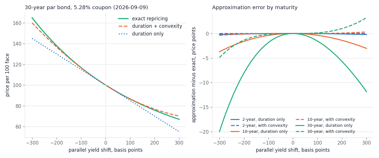
For the 2-year bond the straight line is fine: two tenths of a price point wrong at a 300 basis point move, which almost nothing else in a portfolio would resolve. For the 10-year the error is a third of a point at 100 basis points and between three and four points at 300. For the 30-year bond a 300 basis point fall in yields produces an exact price of 164.93; duration alone predicts 144.92, twenty points short. Adding the convexity term recovers most of it, to 160.01, but is still five points off, and on the other side, at plus 300, the second-order estimate overshoots by three points. The Taylor series is doing exactly what a Taylor series does: it is accurate near the point of expansion and degrades with the cube of the distance from it. Nothing in the second-order formula is wrong; it is just being asked to describe a curve 300 basis points away from where it was fitted, and for a 15-duration bond that is a long way.
The right-hand panel of the figure makes the asymmetry explicit. Duration-only error is always negative and roughly parabolic. The convexity-corrected error changes sign at zero and is small over roughly plus or minus 100 basis points for every maturity shown, which is the range in which the second-order approximation is genuinely useful for the long end of the curve and overkill for the short end.
What twenty-six years of one series does to duration
Duration is a function of the yield as well as the coupon and maturity, and a par bond's coupon changes with the yield, so the interest-rate sensitivity of "a 10-year Treasury" has not been constant. The script evaluates the modified duration of a 10-year par bond at every DGS10 observation since 2000-01-03, all 6,675 of them, and writes the result to datasets/bond-math-price-yield-duration-convexity-history.csv:
| observation | date | DGS10 | modified duration | convexity | DV01 per 100 |
|---|---|---|---|---|---|
| first in the dataset | 2000-01-03 | 6.58% | 7.243 | 66.14 | 0.0724 |
| highest yield | 2000-01-20 | 6.79% | 7.174 | 65.21 | 0.0717 |
| lowest yield | 2020-08-04 | 0.52% | 9.732 | 101.08 | 0.0973 |
| latest | 2026-09-09 | 4.83% | 7.858 | 74.49 | 0.0786 |
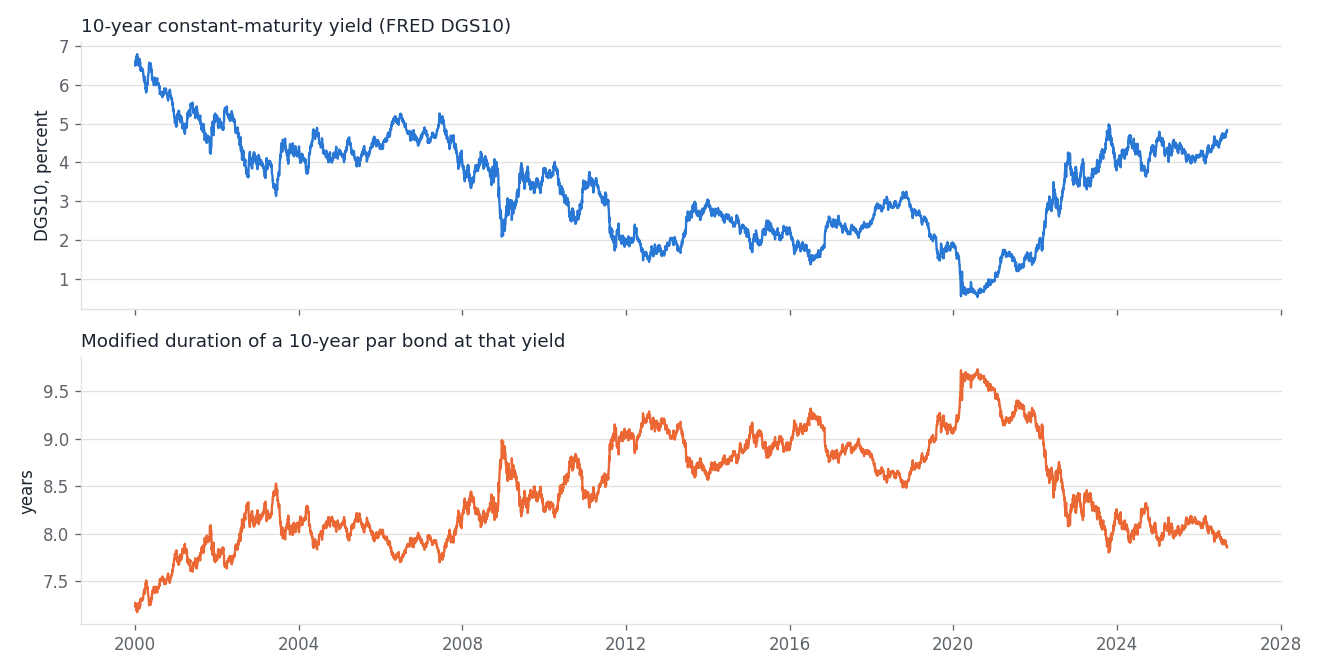
The range is 7.17 to 9.73 years, a 36 percent difference in rate sensitivity for the same maturity, driven entirely by the level of yields. The yearly means make the drift plain: 7.43 in 2000, 8.50 in 2010, 9.55 in 2020, and 8.02 so far in 2026. When the DGS10 print was 0.52 percent on 2020-08-04, a freshly issued par 10-year would have lost about 0.97 percent of its price per ten basis points of yield; at the 2026-09-09 print the same move costs about 0.79 percent. That is a mechanical consequence of the formula, not a statement about what yields will do, and the script prints the whole yearly table so the drift can be inspected rather than summarised.
Reproducibility and limits
datasets/bond-math-price-yield-duration-convexity.csv is the raw pull: date, then one column per series DGS1MO through DGS30, percent per annum, with FRED's "." rendered as an empty cell; DGS1MO begins 2001-07-31 and the others 2000-01-03. -shocks.csv holds 75 rows: curve_date, series, years, coupon_pct, shift_bp, yield_pct, price_exact, price_duration, price_duration_convexity, and the two error columns. -history.csv holds 6,675 rows: date, DGS10_pct, modified_duration_10y_par, convexity_10y_par, dv01_per_100. Run python code/bond-math-price-yield-duration-convexity.py --download --figures to refresh everything including the two charts; the numbers need only the standard library, and the charts need matplotlib 3.10.9.
The limits are the conventions. Every bond here is hypothetical, a par instrument whose coupon equals the quoted yield, with exactly a whole number of semiannual periods to maturity, no accrued interest, and no settlement lag; a real Treasury note between coupon dates needs the actual day count and a dirty-to-clean price adjustment that this script does not perform. The shifts are parallel, meaning every point on the curve moves by the same amount, which is the assumption duration itself makes and which the curve routinely violates: on 2026-09-09 the 2-year sat 40 basis points below the 10-year and the 20-year printed the same yield as the 30-year, and neither of those shapes is a parallel move from the 2000 curve. Bill yields are quoted on an investment basis and we have discounted them with semiannual compounding, which is a simplification of how bills actually trade. One further thing we did not resolve: H.15's footnote 9 says the 30-year constant maturity series "was discontinued on February 18, 2002, and reintroduced on February 9, 2006", with the Treasury publishing an adjustment factor in between, yet the FRED file carries 995 DGS30 observations across that window. We have left those values in the dataset as FRED serves them and have not used them for any figure above; how they were derived is a question for the source, not something to assume. And none of this is a reason to hold or avoid any maturity; it is the arithmetic that any such decision would have to start from.